There's Darcy-Weisbach equation for estimation of a pressure drop inside a tube from its geometry and flow conditions. For circular tube in laminar regime pressure drop is equal to:
$$ \Delta{P} = f_D\frac{L}{d}\rho\frac{V^2}{2} $$
where
\(f_D\) is Darcy friction factor
\(L\) is a length of the tube
\(d\) is a diameter of the tube
\(\rho\) is fluid density
\(V\) is average fluid flow velocity
In the post person was complaining about large difference between pressure drop estimated from Darcy-Weisbach equation and simulation results. As the simulation was rather obvious, and I had tube mesh nearby, so I've executed 3D case and got pressure drop value 12% off the estimation, attributed it to overall mesh quality. Cause its improvement would eventually lead to parallel simulation I've decided to run 2D simulations to check if I can get exact value of pressure drop.
Tube geometry and flow parameters are as follows:
\(L = 5~m\)
\(d = 0.02~m\)
\(\rho = 1000~\dfrac{kg}{m^3}\)
\(\nu = 10^{-6}~\dfrac{m^2}{s}\)
\(V = 0.001~\dfrac{m}{s}\,\,(Re = 20), 0.005~\dfrac{m}{s}\,\,(Re = 100)\)
According to Darcy-Weisbach pressure drop for these cases should be \(dp = 0.4~Pa\) and \(dp = 2~Pa\) correspondingly.
If in 3D there are certain inconvenient things during mesh construction, in axisymmetric 2D it's just a rectangle (though one needs to obey rules of wedge boundaries construction). Cases can be downloaded from GitHub. They are obvious simpleFoam cases with the following SIMPLE dictionary:
SIMPLE
{
    nNonOrthogonalCorrectors 0;

    residualControl
    {
        "(p|k|epsilon)" 1e-6;
        Ux 1e-6;
        Uz 1e-6;
    }
}

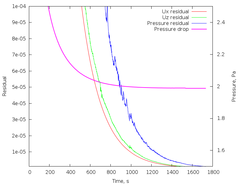
So there were two stages of the solution: initial rapid pressure and residuals drop and further slow convergence to the pressure drop estimated with D-W equation. As the value of the pressure drop seems to be flat after 600 s, below are two zoomed versions of the plot: the first just changes range on y-axis, while the second also changes range on x-axis:


So on zoomed plots one can see that in fact pressure goes slightly below estimated value (guess, due to the way I estimated pressure drop in simulation). Also one can choose desired value of convergence criterion residuals and estimate the error. It would be quite interesting to check this thing in transient simulations as usually people select fixed number of outer iterations instead of residual control for convergence criterion.
The same figures for the case Re = 100 are shown below:

The pressure drop evolution looks almost like in the previous case, though it took longer to converge (due to higher Reynolds number?).

Zoomed versions of the plot again show that pressure drop went below estimated value and flatlining of the pressure is not actually flatlining.
Look out for your residuals.