lundi 10 novembre 2014

Darcy-Weisbach & simpleFoam

The post is a result of this thread at cfd-online.com.

There's Darcy-Weisbach equation for estimation of a pressure drop inside a tube from its geometry and flow conditions. For circular tube in laminar regime pressure drop is equal to:

$$ \Delta{P} = f_D\frac{L}{d}\rho\frac{V^2}{2} $$
where

\(f_D\) is Darcy friction factor

\(L\) is a length of the tube

\(d\) is a diameter of the tube

\(\rho\) is fluid density

\(V\) is average fluid flow velocity

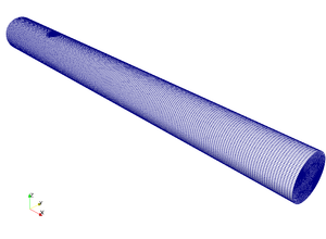
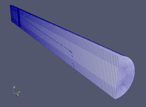
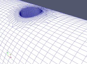
In the post person was complaining about large difference between pressure drop estimated from Darcy-Weisbach equation and simulation results. As the simulation was rather obvious, and I had tube mesh nearby, so I've executed 3D case and got pressure drop value 12% off the estimation, attributed it to overall mesh quality. Cause its improvement would eventually lead to parallel simulation I've decided to run 2D simulations to check if I can get exact value of pressure drop.

Tube geometry and flow parameters are as follows:


\(L = 5~m\)

\(d = 0.02~m\)

\(\rho = 1000~\dfrac{kg}{m^3}\)

\(\nu = 10^{-6}~\dfrac{m^2}{s}\)

\(V = 0.001~\dfrac{m}{s}\,\,(Re = 20), 0.005~\dfrac{m}{s}\,\,(Re = 100)\)

According to Darcy-Weisbach pressure drop for these cases should be \(dp = 0.4~Pa\) and \(dp = 2~Pa\) correspondingly.

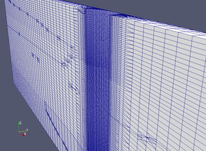
If in 3D there are certain inconvenient things during mesh construction, in axisymmetric 2D it's just a rectangle (though one needs to obey rules of wedge boundaries construction). Cases can be downloaded from GitHub. They are obvious simpleFoam cases with the following SIMPLE dictionary:

SIMPLE
{
    nNonOrthogonalCorrectors 0;

    residualControl
    {
        "(p|k|epsilon)" 1e-6;
        Ux 1e-6;
        Uz 1e-6;
    }
}

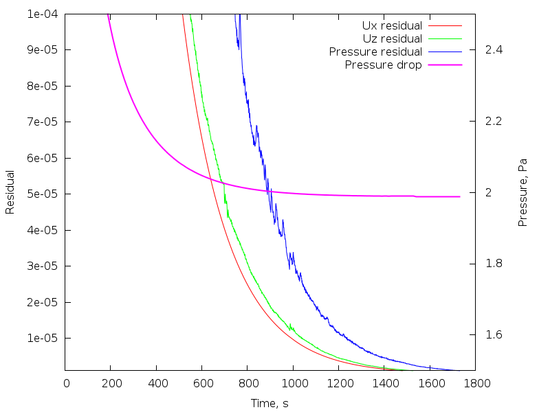
Well, k and epsilon residuals are not necessary for low Reynolds numbers. On figure below overall solution process is displayed. Around 1300 iteration convergence criterion was satisfied and simulation stopped.

So there were two stages of the solution: initial rapid pressure and residuals drop and further slow convergence to the pressure drop estimated with D-W equation. As the value of the pressure drop seems to be flat after 600 s, below are two zoomed versions of the plot: the first just changes range on y-axis, while the second also changes range on x-axis:

So on zoomed plots one can see that in fact pressure goes slightly below estimated value (guess, due to the way I estimated pressure drop in simulation). Also one can choose desired value of convergence criterion residuals and estimate the error. It would be quite interesting to check this thing in transient simulations as usually people select fixed number of outer iterations instead of residual control for convergence criterion.

The same figures for the case Re = 100 are shown below:
The pressure drop evolution looks almost like in the previous case, though it took longer to converge (due to higher Reynolds number?).
Zoomed versions of the plot again show that pressure drop went below estimated value and flatlining of the pressure is not actually flatlining.

Look out for your residuals.

dimanche 20 juillet 2014

Building OpenFOAM on OS X. Update.

As I've got tired of struggling with Blogger (funny layout, lack of ability to markup posts in Markdown, rather inconvenient commenting) I've decided to move patches repository to Github. So all questions and bugs can be filed there. Installation guides can be found in wiki.

Since last post I've added the following things:

  1. Added patches for 2.1.x versions.
  2. Finally I've got a fresh OS X 10.9 installation and found out there's no gdb, so I've added lldb support to addr2line_mac.py. Also cleaned code a bit so it passes pylint without complains.
  3. Changed paraview from alias to function so now paraFoam doesn't complain about unknown command.
  4. Corrected sed patterns in Alltest file from tutorials folder.
  5. Added a sample file for environment setup.
As finally I was able to pass human test on openfoamwiki.net, maybe installation guides there should be also updated.

mardi 15 avril 2014

Building OpenFOAM on OS X

NB. Updated versions of the patches are on Github.

Previous patches I've posted in this blog (#1, #2, #3) have certain mistakes. Mainly because I forgot about DYLD_LIBRARY_PATH environment variable and did not test parallel execution of the solvers. Recently I've decided it is time to fix it. Also that tiny feedback I had, showed that there is two common errors during compilation: people create disk images with case insensitive file system and they try to apply patches in an arbitrary folders. The second problem is hard to solve by a blog post, while the first one can be solved if we change the process of disk image creation. Go from error-prone GUI way to just one command executed in terminal window. And here goes the guide.
Build process was tested on OS X version 10.9.2 with clang --version: Apple LLVM version 5.1 (clang-503.0.38) (based on LLVM 3.4svn).

Before we start

I've made certain assumptions about the software you have on your Mac:
  • Homebrew is used as a package manager to install open source software. If not, you can install it following instructions on the site.
  • All software from ThirdParty source pack will be installed using Homebrew.
  • All commands are executed in Terminal application (usually it is called Terminal.app).
  • $ in the beginning of the lines is a shell prompt and you don't need to copy it, if you're copy/pasting commands from the post. In general commands should be executed in the sequence shown in the post.
  • You've downloaded Paraview application from paraview.org and installed it in /Applications.
To install dependencies you can use the following set of commands:
$ brew tap homebrew/science
$ brew install open-mpi
$ brew install scotch
$ brew install boost --without-single --with-mpi
$ brew install cgal
The last command will also install cmake, gmp, and mpfr as dependencies.

Downloading necessary pieces

At this point it is time to decide what version of OpenFOAM you'd like to build. As 2.3.0 introduced certain backward incompatible changes, I've made patches for 2.2.2 and 2.3.0. Further in the guide I assume you've downloaded source pack and patch into ~/Downloads/OpenFOAM folder.

OpenFOAM 2.2.2

Download source pack. Either following link on the OpenFOAM web site http://www.openfoam.org/archive/2.2.2/download/source.php, or by executing the following commands in in Terminal:
$ cd Downloads
$ mkdir OpenFOAM && cd OpenFOAM
$ curl -L http://downloads.sourceforge.net/foam/OpenFOAM-2.2.2.tgz > OpenFOAM-2.2.2.tgz
Download patch using following link https://raw.githubusercontent.com/mrklein/openfoam-os-x/master/OpenFOAM-2.2.2.patch, or if you still have terminal opened, issue the command:
$ curl -L https://raw.githubusercontent.com/mrklein/openfoam-os-x/master/OpenFOAM-2.2.2.patch > OpenFOAM-2.2.2.patch

OpenFOAM 2.3.0

Download source pack. Either following link on the OpenFOAM web site - http://www.openfoam.org/download/source.php, or just executing this in Terminal:
$ cd Downloads
$ mkdir OpenFOAM && cd OpenFOAM
$ curl -L http://downloads.sourceforge.net/foam/OpenFOAM-2.3.0.tgz > OpenFOAM-2.3.0.tgz
Download patch using following link https://raw.githubusercontent.com/mrklein/openfoam-os-x/master/OpenFOAM-2.3.0.patch, or if you still have terminal opened issue the command:
$ curl -L https://raw.githubusercontent.com/mrklein/openfoam-os-x/master/OpenFOAM-2.3.0.patch > OpenFOAM-2.3.0.patch
After this you're ready to proceed to the actual build process.

Building OpenFOAM

!!! Cause certain file names in this part depend on the version of OpenFOAM you're building, I use N and M variables in the file names. For OpenFOAM version 2.2.2: N=2, M=2; for OpenFOAM version 2.3.0: N=3, M=0.

Also it is possible that you already have disk image with the same name in your home folder. Correct the names accordingly.


To build OpenFOAM first you need to create disk image with case sensitive file system. You can either follow the guide from OpenFOAM wiki, or just issue these commands in your terminal:
$ cd
$ hdiutil create -size 4.4g -type SPARSEBUNDLE -fs HFSX -volname OpenFOAM -fsargs -s OpenFOAM.sparsebundle
Last command will create disk image with the name OpenFOAM.sparsebundle with estimated size 4.4 G (as it is the sparse image, after creation the size of the file will be different), create HFS+ file system with a volume name OpenFOAM in the image. Finally -fsargs -s will instruct newfs_hfs utility to create case sensitive file system.
After the image was created you can mount it, I will assume it is mounted in $HOME/OpenFOAM
$ mkdir OpenFOAM
$ hdiutil attach -mountpoint $HOME/OpenFOAM OpenFOAM.sparsebundle
After you extract source pack, copy patch to the created folder, and apply patch (remember, you've downloaded the source pack and the patch into ~/Downloads/OpenFOAM):
$ cd OpenFOAM
$ tar xzf ~/Downloads/OpenFOAM/OpenFOAM-2.N.M.tgz
$ cd OpenFOAM-2.N.M
$ cp ~/Downloads/OpenFOAM/OpenFOAM-2.N.M.patch .
$ git apply OpenFOAM-2.N.M.patch
At this point maybe you'll need to edit etc/bashrc file. But since compiler settings are fixed (it is Clang), OpenMPI and other libraries settings are fixed (they are installed with Homebrew), in fact the only thing worth editing is path settings and only in case if you're installing OpenFOAM elsewhere (i.e. not in $HOME/OpenFOAM). Now you're more-or-less ready to compile.
$ source etc/bashrc
$ ./Allwmake > log.Allwmake 2>&1
The last command executes Allwmake script and redirects its output to log.Allwmake file; just in case, if anything goes wrong, it'll be easy to locate the source of error having this log file.
After Allwmake execution is finished, you can test the build with:
$ mkdir -p $FOAM_RUN
$ run
$ cp -r $FOAM_TUTORIALS/incompressible/icoFoam/cavity .
$ cd cavity
$ blockMesh
$ icoFoam
If you'd like to test parallel run, it is necessary to do:
$ cat > system/decomposeParDict
/*--------------------------------*- C++ -*----------------------------------*\
| =========                 |                                                 |
| \\      /  F ield         | OpenFOAM: The Open Source CFD Toolbox           |
|  \\    /   O peration     | Version:  2.3.0                                 |
|   \\  /    A nd           | Web:      www.OpenFOAM.org                      |
|    \\/     M anipulation  |                                                 |
\*---------------------------------------------------------------------------*/
FoamFile
{
    version     2.0;
    format      ascii;
    class       dictionary;
    location    "system";
    object      decomposeParDict;
}
// * * * * * * * * * * * * * * * * * * * * * * * * * * * * * * * * * * * * * //

numberOfSubdomains 4;

method          scotch;
^D
$ decomposePar
$ mpiexec -np 4 icoFoam -parallel
(^D is entered with Ctrl and D keys pressed together)

Post-configuration

There are several ways of managing mounting disk image and sourcing etc/bashrc file.
The first one is to define alias in your $HOME/.profile:
alias of2NM='hdiutil attach -quiet -mountpoint $HOME/OpenFOAM OpenFOAM.sparsebundle; sleep 1; source $HOME/OpenFOAM/OpenFOAM-2.N.M/etc/bashrc'
The second one is to create $HOME/.OpenFOAM-release file with a version of OpenFOAM you'd like to use:
$ echo '2.N.M' > $HOME/.OpenFOAM-release
and then add the following lines to your $HOME/.profile:
if [ -f $HOME/.OpenFOAM-release ]; then
        OF_VER=$(cat $HOME/.OpenFOAM-release)
        if [ ! -f $HOME/OpenFOAM/OpenFOAM-$OF_VER/etc/bashrc ]; then
                hdiutil attach -quiet -mountpoint $HOME/OpenFOAM OpenFOAM.sparsebundle && . $HOME/OpenFOAM/OpenFOAM-$OF_VER/etc/bashrc
        else
                . $HOME/OpenFOAM/OpenFOAM-$OF_VER/etc/bashrc
        fi
fi
And finally third one is to transform second version in the set of functions. I.e. instead of automatic attachment of disk image upon terminal start, you'll need to execute function which will mount necessary disk image and source bashrc:

of2xx() {
    local version=$1
    if [ ! -f $HOME/OpenFOAM/OpenFOAM-$version/etc/bashrc ]; then
        hdiutil attach -quiet -mountpoint $HOME/OpenFOAM OpenFOAM.sparsebundle &&
            . $HOME/OpenFOAM/OpenFOAM-$version/etc/bashrc
    else
        . $HOME/OpenFOAM/OpenFOAM-$version/etc/bashrc
    fi
}

of2NM() {
    of2xx '2.N.M'
}
Add this code to your $HOME/.profile and use of2NM command to setup environment.

And that's it.

mardi 18 mars 2014

Plotting VTK files with matplotlib and python-vtk

Paraview is good. But pictures produced by the software is in general raster (maybe I can't use it right but even if I build with gl2ps I can't find a way to export scene to PS or PDF). So usually I used sample utility to write a slice of interest to a RAW file, then load it with numpy and then use tricontourf to produce color map of a value. And then I can save it as a PDF (or EPS, or PS) so the figure can be scaled without quality loss.

Everything is good (though there's certain problems with matplotlib's triangulation sometimes) but in this case I had a hole in a flow field. So if I have a file with (x, y, value) tuples, the hole will be also triangulated with a value equal to zero and a final tricontourf figure will be quite far from the original flow field. Also as OpenFOAM's sample utility will anyway create a triangulation of the mesh, why do it again. So I've decided to try plotting VTK file with a triangular grid. And it was more or less easy. Though there's almost no documentation on python-vtk module. Well, I guess this module is just a wrapper around C++ so one need to write C++-python instead of python.

Surely this script can be improved to handle vectors and scalars automatically, to handle polymesh files in more general way (currently I suppose, all polygons in the mesh are triangles).
Here is a script for loading a vector field and plotting its X component:

#!/usr/bin/env python

import numpy as N
import vtk
import matplotlib.pyplot as P

def load_velocity(filename):
    if not os.path.exists(filename): return None
    reader = vtk.vtkPolyDataReader()
    reader.SetFileName(filename)
    reader.ReadAllVectorsOn()
    reader.Update()

    data = reader.GetOutput()
    cells = data.GetPolys()
    triangles = cells.GetData()
    points = data.GetPoints()
    point_data = data.GetPointData()
    Udata = point_data.GetArray(0)

    ntri = triangles.GetNumberOfTuples()/4
    npts = points.GetNumberOfPoints()
    nvls = Udata.GetNumberOfTuples()

    tri = N.zeros((ntri, 3))
    x = N.zeros(npts)
    y = N.zeros(npts)
    ux = N.zeros(nvls)
    uy = N.zeros(nvls)

    for i in xrange(0, ntri):
        tri[i, 0] = triangles.GetTuple(4*i + 1)[0]
        tri[i, 1] = triangles.GetTuple(4*i + 2)[0]
        tri[i, 2] = triangles.GetTuple(4*i + 3)[0]

    for i in xrange(points.GetNumberOfPoints()):
        pt = points.GetPoint(i)
        x[i] = pt[0]
        y[i] = pt[1]

    for i in xrange(0, Udata.GetNumberOfTuples()):
        U = Udata.GetTuple(i)
        ux[i] = U[0]
        uy[i] = U[1]

    return (x, y, tri, ux, uy)

P.clf()
levels = N.linspace(-0.5, 1.5, 64)
x, y, tri, ux, uy = load_velocity('U-file.vtk')
P.tricontour(x, y, tri, ux, levels, linestyles='-',
             colors='black', linewidths=0.5)
P.tricontour(x, y, tri, ux, levels)
P.gca().set_aspect('equal')
P.minorticks_on()
P.gca().set_xticklabels([])
P.gca().set_yticklabels([])
P.title('$U_x$ / Gamma')
P.savefig("Ux.png", dpi=300, bbox_inches='tight')
P.savefig("Ux.pdf", bbox_inches='tight')

(Note: updated version of the script adapted for VTK 6.2.0 is posted here)

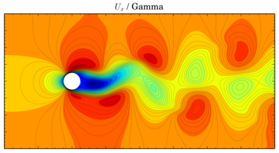
And as a result of this script we'll get this nice picture:

image

And here is a link to the genereated PDF.

OpenFOAM, residuals, and vortex street

This post appeared due to the question on cfd-online.com OpenFOAM forum. It has been started as yet another post on Kármán vortex street but then (around message #60) original poster revealed an article he was trying to compare with, so I've decided to check influence of different discretisation schemes and convergence criterions on final results.

Geometry and flow conditions

The first version of geometry and boundary conditions can be found in post #11, though they slightly differ from the geometry provided in the article (and as a result, from geometry used in simulations).


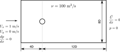
So we've got a cylinder with diameter D placed in the channel with a length 16D and a width 8D. At the inlet we have velocity 1 m/s, at the outlet zero pressure and zero gradient in velocity. Initially velocity inside the domain set to 1 m/s. With D = 1 m and fluid kinematic viscosity 100 m2/s, Reynolds number is equal to 100.

First attempt

Well, the first variant of the simulation was just a simulation for its own sake (even Re was 200). Just to produce neat pictures. And these videos:


Flow develops, vortices go.

Second attempt

After reading the original article I've decided to check different meshes, discretisation schemes, and convergence criteria to learn if there's any difference. In the article authors were developing new method in FEM framework, so theirs original mesh was triangular with increased density near a centerline of the channel. Now I think there's a need for another set of simulations: with and without increase of mesh density near the center-line of the channel.

Meshes

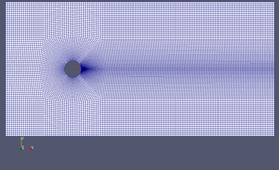
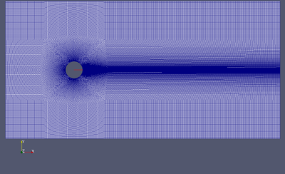
I've fallen in love with Gmsh for generating meshes, so these two meshed are produced with it. As Gmsh now has transfinite algorithm, it is more or less like blockMesh with GUI, variables and functions in a mesh file, more convenient way of grading description. Much like in blockMesh one needs to define vertices and then can use GUI to describe lines, surfaces and volumes. Then again switch to text editor for definition of transfinite lines, progressions (in the sense of Gmsh), etc. I will omit iterations during the mesh creation process and just provide GEO files with screenshots of the mesh:
"Coarse" mesh

image
Coarse cylinder-2D.geo

"Fine" mesh

image
Fine cylinder-2D.geo

The only difference between coarse and fine mesh is twice increased density in case of "Fine" mesh. So a number of cells in the fine mesh is 4 times higher than in coarse mesh.

fvSchemes

Typical fvSchemes file is provided below. The only line that is changed from simulation to simulation is div(phi,U) Gauss vanLeerV;, I've chosen to compare three different second order discretisation schemes with limiters: van Leer, QUICK, and Gamma.

/*--------------------------------*- C++ -*----------------------------------*\
| =========                 |                                                 |
| \\      /  F ield         | OpenFOAM: The Open Source CFD Toolbox           |
|  \\    /   O peration     | Version:  1.6                                   |
|   \\  /    A nd           | Web:      www.OpenFOAM.org                      |
|    \\/     M anipulation  |                                                 |
\*---------------------------------------------------------------------------*/
FoamFile
{
   version     2.0;
   format      ascii;
   class       dictionary;
   location    "system";
   object      fvSchemes;
}
// * * * * * * * * * * * * * * * * * * * * * * * * * * * * * * * * * * * * * //

ddtSchemes
{
   default         CrankNicolson 1.0;
}

gradSchemes
{
   default         Gauss linear;
}

divSchemes
{
   default         none;
   div(phi,U)      Gauss vanLeerV;
   div((nuEff*dev(T(grad(U))))) Gauss linear;
}

laplacianSchemes
{
   default         none;
   laplacian(nuEff,U) Gauss linear corrected;
   laplacian((1|A(U)),p) Gauss linear corrected;
}

interpolationSchemes
{
   default         linear;
}

snGradSchemes
{
   default         corrected;
}

fluxRequired
{
   default         no;
   p               ;
}


// ************************************************************************* //

fvSolution

In case of fvSolution file I changed PIMPLE dictionary:
PIMPLE
{
    momentumPredictor yes;
    nCorrectors       2;
    nOuterCorrectors  20;
    nNonOrthogonalCorrectors 1;

    residualControl
    {
        "(U|p)"
        {
            tolerance 1e-2;
            relTol 0;
        }
    }
}

Keeping everything else the same, I changed tolerance in residualControl dictionary to see if it influence results. I've checked values 1e-2, 1e-4, and 1e-6. This value defines the moment when PIMPLE loop will exit from outer corrector cycle. And usually in the beginning of a simulation number of outer correctors is around 4 (for the case of residual 1e-6 - 8), during the time this number falls to 2 (or 4 for the case of 1e-6). I don't know why all tutorial cases use fixed number of outer corrector iterations, sometimes it can lead to completely incorrect results. Maybe OpenFOAM decided that residualControl is "advanced" technique.

Also there're lots of scary posts on relaxation, so I've decided also to check the influence of relaxation factors on results of a simulation. So instead of standard

relaxationFactors
{
    fields
    {
    }
    equations
    {
       "U.*" 1.0;
       "p.*" 1.0;
    }
}

I used

relaxationFactors
{
    fields
    {
    }
    equations
    {
       "U.*" 0.7;
       "p.*" 0.3;
    }
}

Results

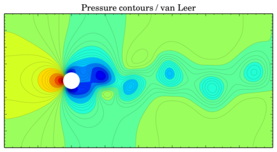
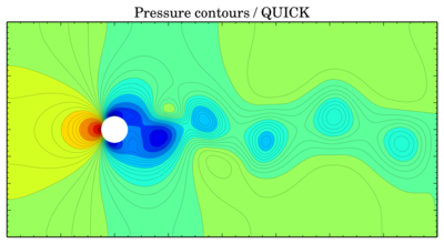
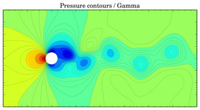
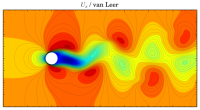
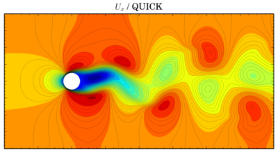
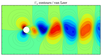
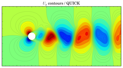
Color contours usually provide only schematic view of the flow, so further (surely after these pictures) I will be comparing oscillations of force coefficients. Sometimes it is possible to plot isolines of pressure and velocity on the same picture (when the phases of the oscillating flow do not differ much). But now, the color contours (time is 150 s):

Pressure
van Leer
image

QUICK
image

Gamma
image

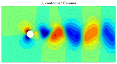
Though values seem to be more or less the same, vortices are shifted in time. The same thing is for velocity components:

Ux
van Leer
image

QUICK
image

Gamma
image

Uy
van Leer
image

QUICK
image

Gamma
image

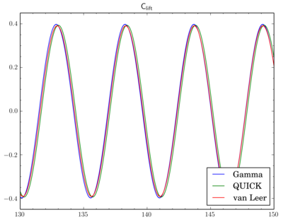
Discretisation schemes comparison

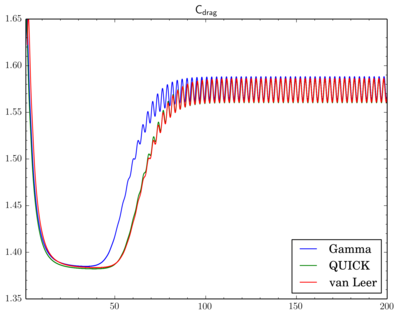
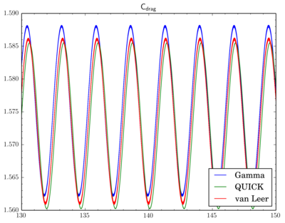
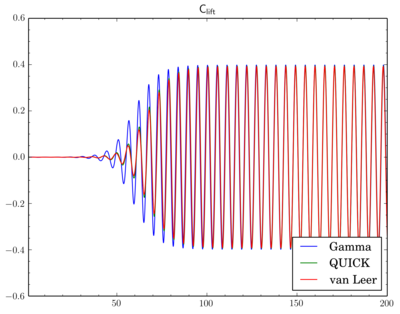
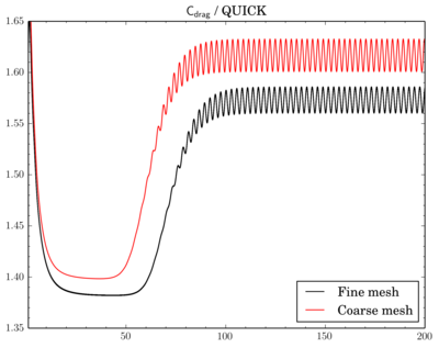
I've fixed final residual in fvSolution at 1e-6 and just changed discretisation scheme. On the graphs X-axis is time, Y-axis is value. All simulations were done on the 'fine' mesh.


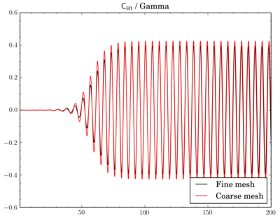
There is phase shift between graphs, I've moved them to compare oscillation amplitude. There is difference but it's not so big.


And as there is phase shift between different scheme I will omit comparison of the pressure and velocity contours. While there is difference between Cdrag oscillation amplitudes, Clift oscillations go rather synchronously:


Final residuals comparison

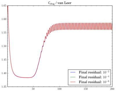
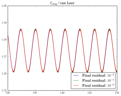
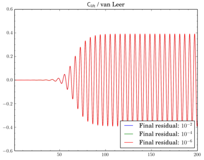
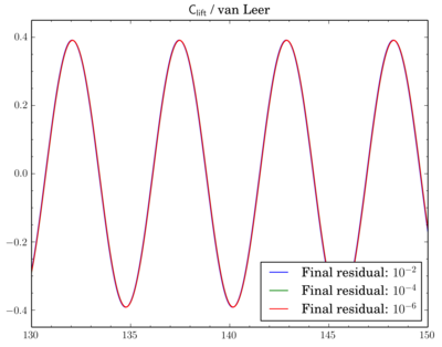
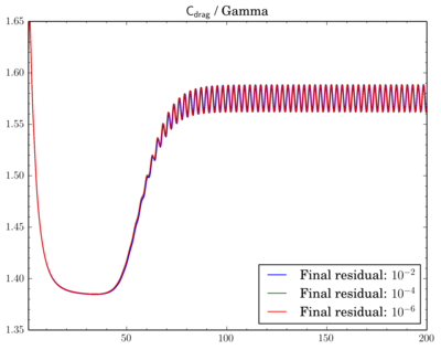
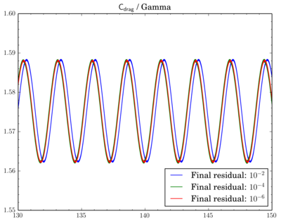
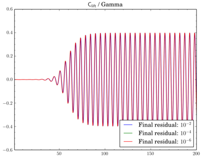
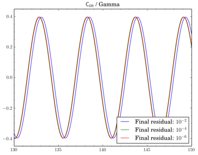
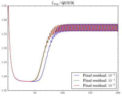
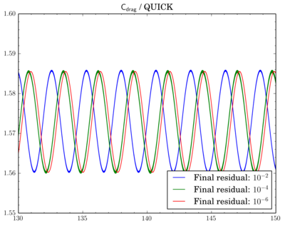
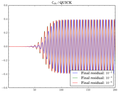
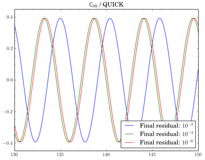
After that I've decided to check sensitivity of a discretisation scheme on final residual. I've fixed the scheme and run simulations for different final residuals: 1e-2, 1e-4, and 1e-6.
While van Leer and Gamma showed almost no dependence (though there is slight shift when going from 1e-2 to 1e-4 for Gamma):


For QUICK switch from 1e-2 to 1e-4 leads to quite large time shift between oscillations:


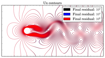
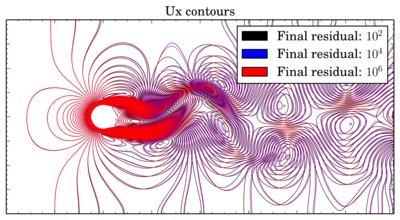
But even if the time shift in oscillations seems to be not so big, positions of the vortices are strongly depend on this shift. Below is overlays of Ux isolines for van Leer and Gamma schemes at 150 s:


If for van Leer scheme contours are almost the same, for Gamma results with residual 1e-2 are sufficiently shifted.
Mesh density comparison

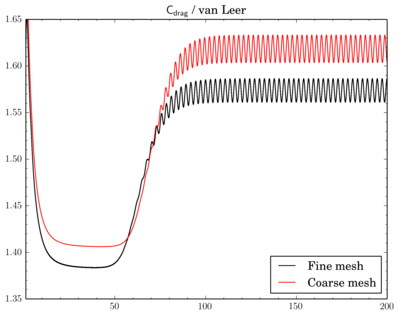
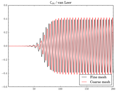
Also compared results acquired using meshes with different densities. Number of cells in the meshes differ 4 times as I've reduced densities twice in X and Y directions.
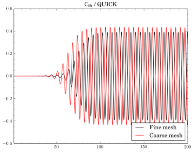
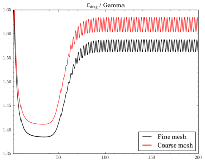
Gamma showed just decrease of Cdrag and Clift values on fine mesh, while with QUICK and van Leer schemes there's also phase shift between results on different meshes.

Cdrag


Clift


To relax or not

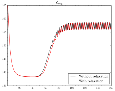
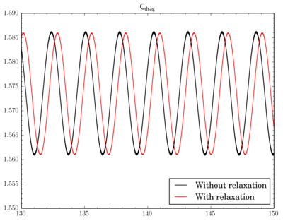
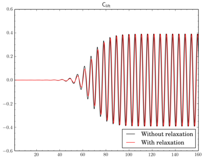
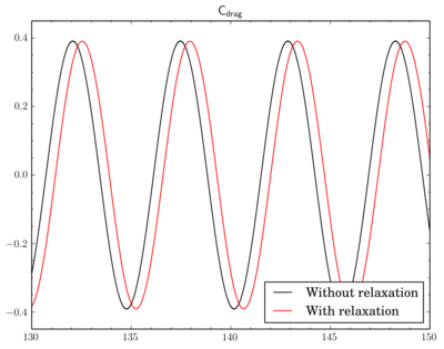
Finally I've decided to check if a relaxation is really crucial to results. I've fixed the discretisation scheme (van Leer, though now I think maybe it was better to choose Gamma), the final residual in PIMPLE dictionary and just modified relaxation part as shown in the beginning of the post. Surely due to the relaxation solution converges slowly, i.e. instead of 4-5 outer corrector iterations 9-11 iterations was necessary. Also there is a time shift between results.


Conclusion

So it goes.

As usual case files (if you'd like to reproduce results) are on bitbucket.org.

samedi 1 mars 2014

Let's put something in a tube

Introduction

After I've done simulations of vortex street in 2D, I kept thinking that it would be nice to do more or less the same thing in 3D. And after watching the movie about vortex flow meters by Endress+Hauser, I've decided it would be really funny to put something in a tube and watch vortices going by.

First of all we need to decide on operational parameters of the system. Let's assume that we have 10 m long tube with diameter of 1 m and let's install something at 2 m from inlet plane. Further calculations are based upon the article from Wikipedia about Kármán vortex street.
Re = uD/ν
where u is flow velocity, D is characteristic length, and ν is fluid viscosity. We'll get vortex street for Re values larger than 90. If we take, for example, water with nu around 1000000 it's not hard to get large enough Reynolds number. But then a question of the distance between vortices arises. We also want our vortices inside the tube. Vortex shedding frequency is
f = 0.198*u/d*(1 - 19.7/Re)
where d is cylinder diameter (correct for 250 < Re < 10^5). After playing with tube and cylinder sizes, fluid viscosity and inflow velocities (here is a script) I've decided to go with the following:
D = 1 m
d = 0.2 m
u = 1 m/s
ν = 0.0001 m^2/s

Meshing

For meshing I've used Gmsh and snappyHexMesh. I.e. I've created hexagonal mesh of the tube, then I've created triangular surface mesh for the cylinder and sphere, a nd finally I've used snappyHexMesh to cut small cylinder (or sphere) tube.

Mesh for tube is based upon my previous post. The addition is a parametrization of the GEO file, i.e. one need to set tube leng th and its diameter; gmsh will recalculate positions of the points in the mesh. GEO files for cutting shapes (cylinder, sphere) are even simpler cause we need only triangular surface mesh so there's no need to split a shape into volumes with 6 sides (this operation necessary for transfinite algorithm to work).

One of the problems I've encountered during "cutting" procedure is the need to use more or less cubical mesh for sHM to work. In case of sphere it wan't actually a problem, cause it lies inside "inner" part of the mesh which is rather regular. So one can have graded mesh near the walls of the tube. That was not so in case on cylinder. After several unsuccessful attempts to cut a cylinder hole in graded mesh (though sHM tried to do it but wasn't able to generate acceptable quality mesh, usually non-orthogonality on the new mesh was too high), I've removed grading.
snappyHexMeshDict is quite simple, first I define the surface:
geometry
{
    sphere.stl
    {
        type triSurfaceMesh;
        name sphere;
    }
};
then I refine mesh around the surface
refinementRegions
{
    sphere
    {
        mode distance;
        levels ((0.05 3) (0.1 2) (0.2 1));
    }
}
refinement is based upon distance from the mesh. Other parameters in the dictionary is just a copy from tutorial.

So after running mesh conversion (from gmsh to OpenFOAM) and then running snappyHexMesh, I've got the following meshes for the simulation:

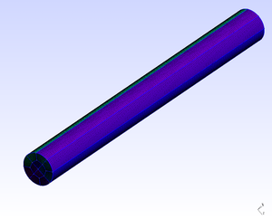
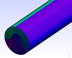
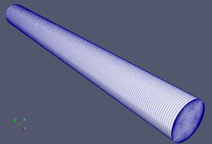
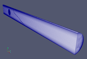
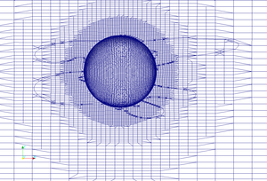
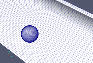
Initial tube mesh


with grading towards the walls


without grading


Mesh with internal cylinder


Mesh with internal sphere


Unlike previous time I've decided not to compare turbulence models and just selected realizable k-epsilon.

Flow movies

After running the simulations I've got the following flow movies:

The cylinder in the tube, vorticity


The cylinder in the tube, velocity


The sphere in the tube, vorticity


The sphere in the tube, velocity


As expected after initial flow development I've got quite nice vortices going along the tube.

Probes

Since the movies are not quite enough I've added probes along the axis of the tube to record values of velocity, pressure, and turbulent viscosity during the simulations (this is a fragment of controlDict):

functions
{
    probes
    {
        type            probes;
        functionObjectLibs ("libsampling.so");
        outputControl   timeStep;
        outputInterval  1;
        probeLocations
        (
            (2.47 0 0)
            (2.90 0 0)
            (3.5 0 0)
            (5 0 0)
            (6 0 0)
        );
        fields
        (
            U
            p
            nut
        );
    }
}

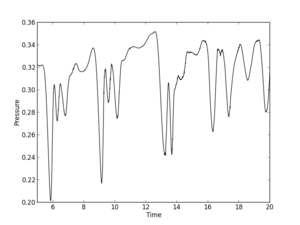
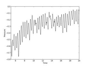
Below is a graphs of the pressure evolution at the location of the first probe (click on the figure for a larger version):

For internal cylinder


For internal sphere


Though evolution has periodic structure but the frequency differs from estimations.

How to run the cases on your own

I've put all necessary files into repository on BitBucket. So you can clone the repo or just download archive of the default branch. There is Cases folder where case files reside. Every case directory has Allprepare script which will do all the necessary utility invocations:

#!/bin/sh
cd ${0%/*} || exit 1

. $WM_PROJECT_DIR/bin/tools/RunFunctions

gmsh - tube.geo
gmsh - cylinder.geo
sed -i -e "s/Created by Gmsh/cylinder/" cylinder.stl
mv cylinder.stl constant/triSurface
gmshToFoam tube.msh
cp -r 0.org 0
changeDictionary
surfaceFeatureExtract
snappyHexMesh -overwrite

The script assumes that you have gmsh in your $PATH and first it creates mesh for tube and cylinder, then corrects STL file created by Gmsh, then places STL files to the directory where sHM will look for it, converts tube mesh to OpenFOAM format, corrects boundary type for walls, and finally runs sHM for final mesh creation. sHM procedure is rather lengthy and needs RAM as the limit on the number of cells is 1500000.