Darcy-Weisbach & simpleFoam

The post is a result of this thread at cfd-online.com.

There's Darcy-Weisbach equation for estimation of a pressure drop inside a tube from its geometry and flow conditions. For circular tube in laminar regime pressure drop is equal to:

$$ \Delta{P} = f_D\frac{L}{d}\rho\frac{V^2}{2} $$
where

\(f_D\) is Darcy friction factor

\(L\) is a length of the tube

\(d\) is a diameter of the tube

\(\rho\) is fluid density

\(V\) is average fluid flow velocity

In the post person was complaining about large difference between pressure drop estimated from Darcy-Weisbach equation and simulation results. As the simulation was rather obvious, and I had tube mesh nearby, so I've executed 3D case and got pressure drop value 12% off the estimation, attributed it to overall mesh quality. Cause its improvement would eventually lead to parallel simulation I've decided to run 2D simulations to check if I can get exact value of pressure drop.

Tube geometry and flow parameters are as follows:


\(L = 5~m\)

\(d = 0.02~m\)

\(\rho = 1000~\dfrac{kg}{m^3}\)

\(\nu = 10^{-6}~\dfrac{m^2}{s}\)

\(V = 0.001~\dfrac{m}{s}\,\,(Re = 20), 0.005~\dfrac{m}{s}\,\,(Re = 100)\)

According to Darcy-Weisbach pressure drop for these cases should be \(dp = 0.4~Pa\) and \(dp = 2~Pa\) correspondingly.

If in 3D there are certain inconvenient things during mesh construction, in axisymmetric 2D it's just a rectangle (though one needs to obey rules of wedge boundaries construction). Cases can be downloaded from GitHub. They are obvious simpleFoam cases with the following SIMPLE dictionary:

SIMPLE
{
    nNonOrthogonalCorrectors 0;

    residualControl
    {
        "(p|k|epsilon)" 1e-6;
        Ux 1e-6;
        Uz 1e-6;
    }
}

Well, k and epsilon residuals are not necessary for low Reynolds numbers. On figure below overall solution process is displayed. Around 1300 iteration convergence criterion was satisfied and simulation stopped.

So there were two stages of the solution: initial rapid pressure and residuals drop and further slow convergence to the pressure drop estimated with D-W equation. As the value of the pressure drop seems to be flat after 600 s, below are two zoomed versions of the plot: the first just changes range on y-axis, while the second also changes range on x-axis:

So on zoomed plots one can see that in fact pressure goes slightly below estimated value (guess, due to the way I estimated pressure drop in simulation). Also one can choose desired value of convergence criterion residuals and estimate the error. It would be quite interesting to check this thing in transient simulations as usually people select fixed number of outer iterations instead of residual control for convergence criterion.

The same figures for the case Re = 100 are shown below:

The pressure drop evolution looks almost like in the previous case, though it took longer to converge (due to higher Reynolds number?).

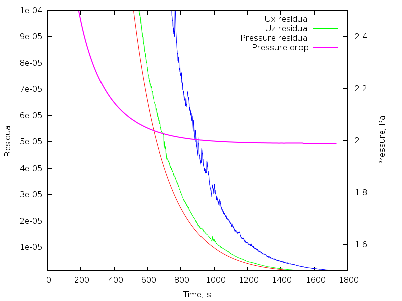
Zoomed versions of the plot again show that pressure drop went below estimated value and flatlining of the pressure is not actually flatlining.

Look out for your residuals.

Let's put something in a tube

Introduction

After I've done simulations of vortex street in 2D, I kept thinking that it would be nice to do more or less the same thing in 3D. And after watching the movie about vortex flow meters by Endress+Hauser, I've decided it would be really funny to put something in a tube and watch vortices going by.

First of all we need to decide on operational parameters of the system. Let's assume that we have 10 m long tube with diameter of 1 m and let's install something at 2 m from inlet plane. Further calculations are based upon the article from Wikipedia about Kármán vortex street.

Re = uD/ν

where u is flow velocity, D is characteristic length, and ν is fluid viscosity. We'll get vortex street for Re values larger than 90. If we take, for example, water with nu around 1000000 it's not hard to get large enough Reynolds number. But then a question of the distance between vortices arises. We also want our vortices inside the tube. Vortex shedding frequency is

f = 0.198*u/d*(1 - 19.7/Re)

where d is cylinder diameter (correct for 250 < Re < 10^5). After playing with tube and cylinder sizes, fluid viscosity and inflow velocities (here is a script) I've decided to go with the following:

D = 1 m
d = 0.2 m
u = 1 m/s
ν = 0.0001 m^2/s

Meshing

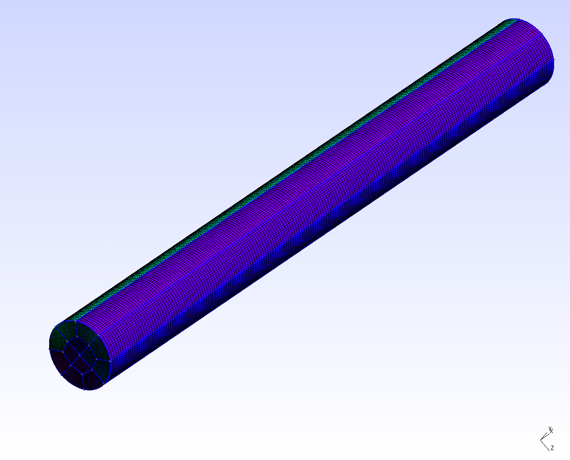
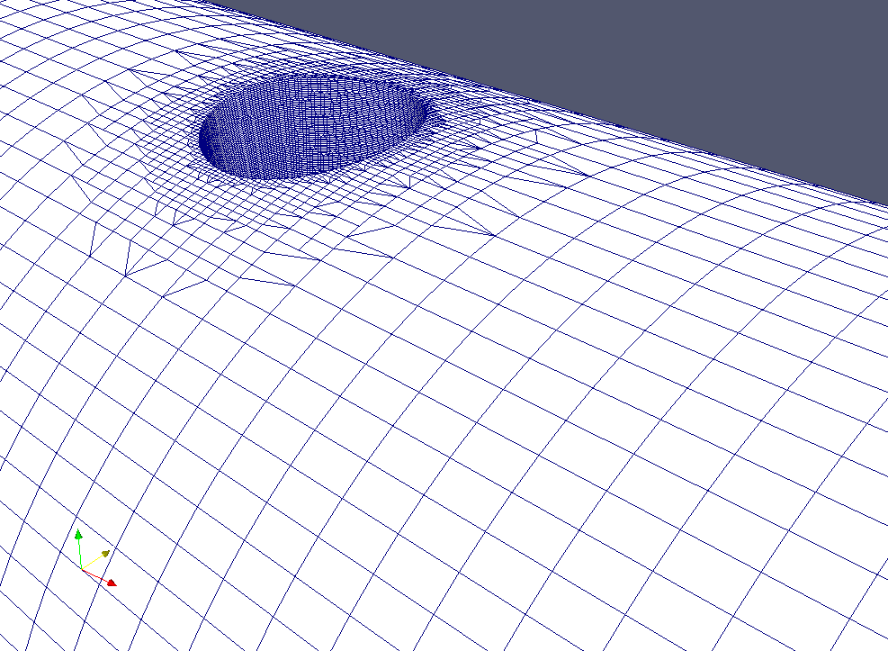
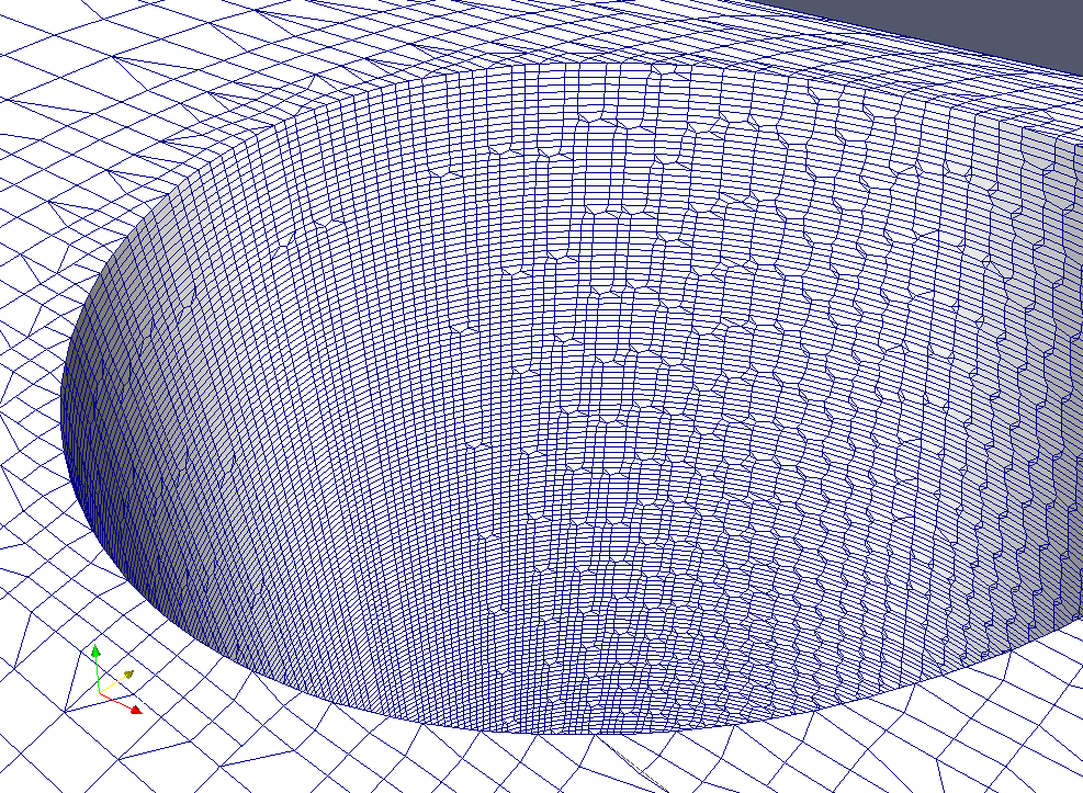
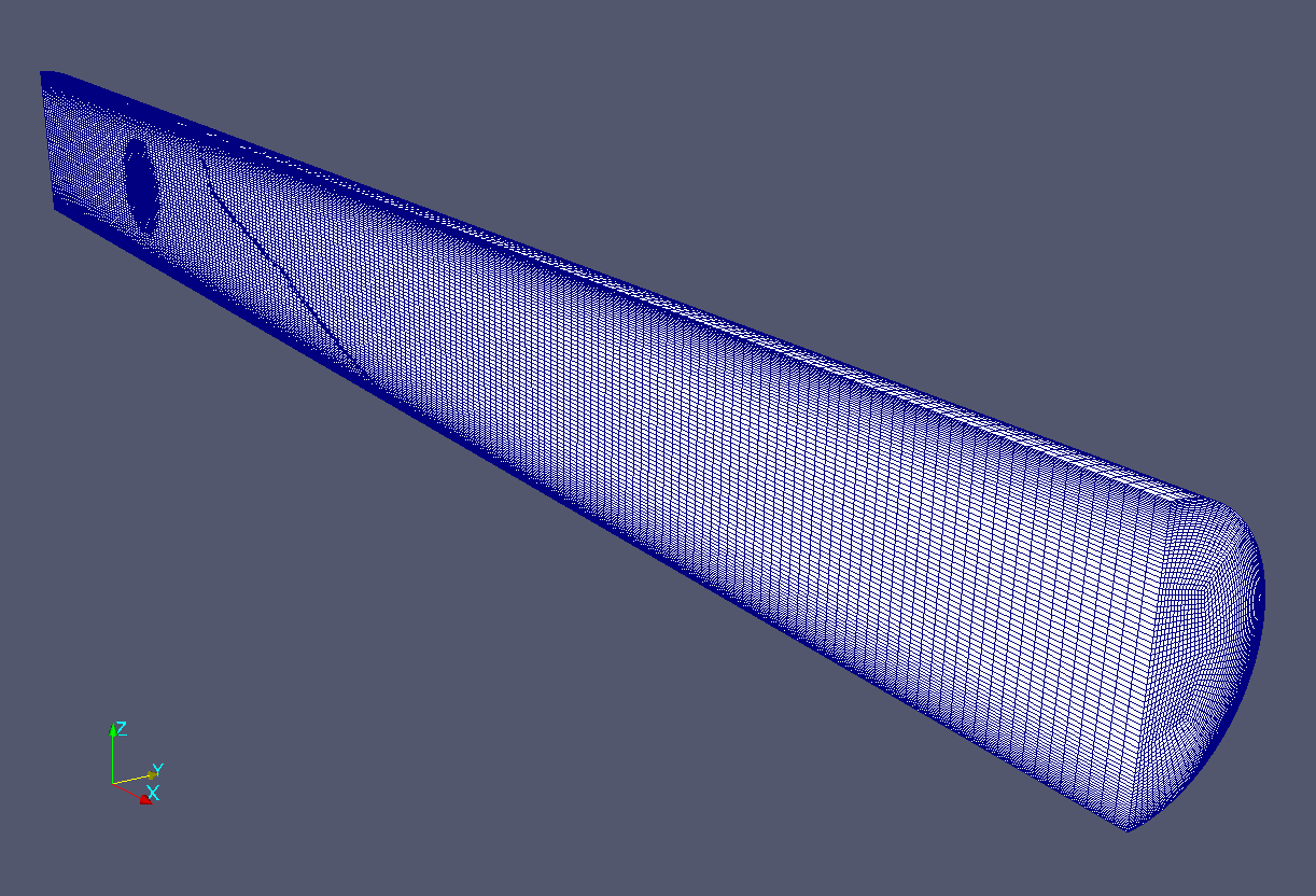
For meshing I've used Gmsh and snappyHexMesh. I.e. I've created hexagonal mesh of the tube, then I've created triangular surface mesh for the cylinder and sphere, a nd finally I've used snappyHexMesh to cut small cylinder (or sphere) tube.

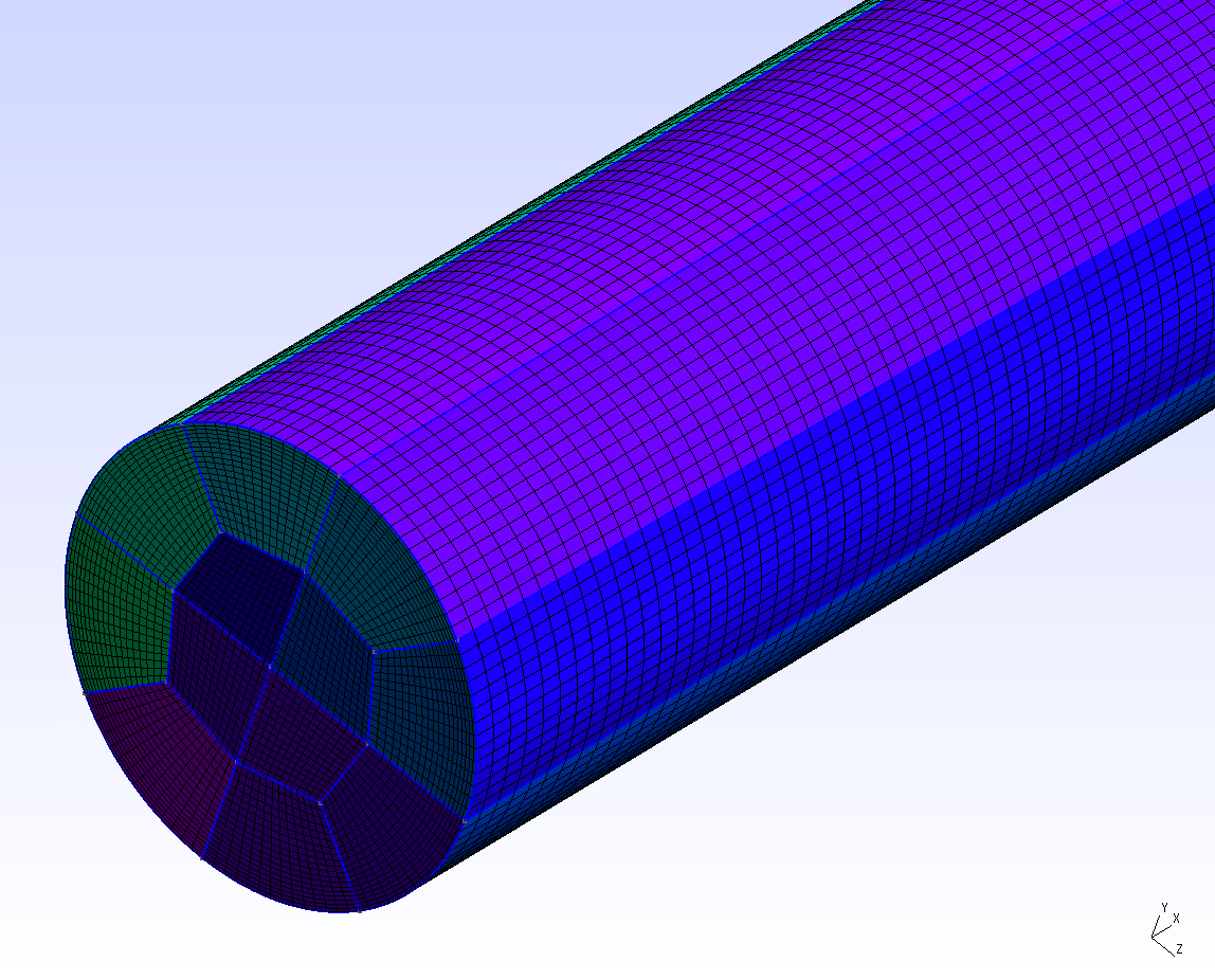
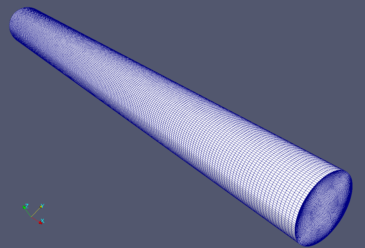
Mesh for tube is based upon my previous post. The addition is a parametrization of the GEO file, i.e. one need to set tube leng th and its diameter; gmsh will recalculate positions of the points in the mesh. GEO files for cutting shapes (cylinder, sphere) are even simpler cause we need only triangular surface mesh so there's no need to split a shape into volumes with 6 sides (this operation necessary for transfinite algorithm to work).

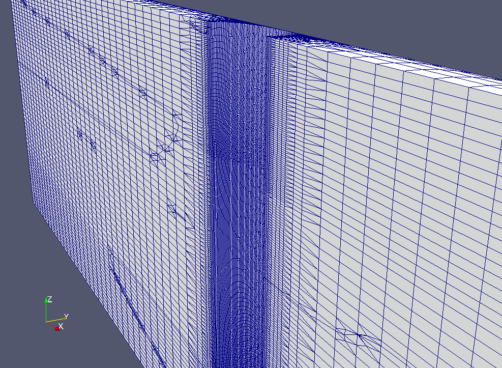
One of the problems I've encountered during "cutting" procedure is the need to use more or less cubical mesh for sHM to work. In case of sphere it wan't actually a problem, cause it lies inside "inner" part of the mesh which is rather regular. So one can have graded mesh near the walls of the tube. That was not so in case on cylinder. After several unsuccessful attempts to cut a cylinder hole in graded mesh (though sHM tried to do it but wasn't able to generate acceptable quality mesh, usually non-orthogonality on the new mesh was too high), I've removed grading.
snappyHexMeshDict is quite simple, first I define the surface:

geometry
{
    sphere.stl
    {
        type triSurfaceMesh;
        name sphere;
    }
};

then I refine mesh around the surface

refinementRegions
{
    sphere
    {
        mode distance;
        levels ((0.05 3) (0.1 2) (0.2 1));
    }
}

refinement is based upon distance from the mesh. Other parameters in the dictionary is just a copy from tutorial.

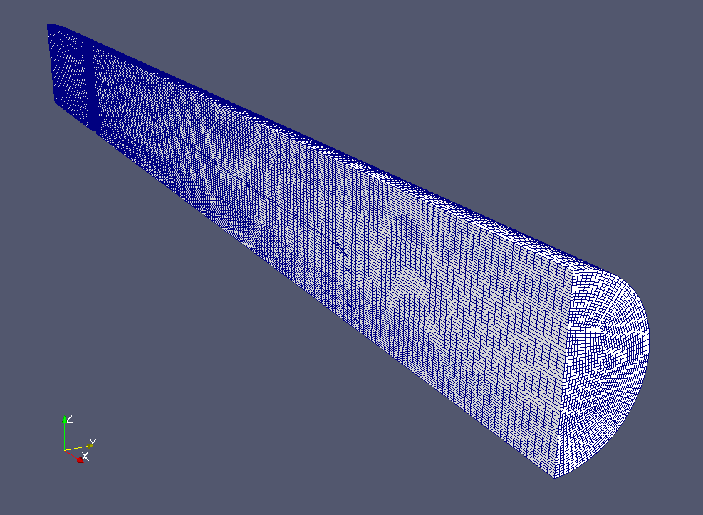
So after running mesh conversion (from gmsh to OpenFOAM) and then running snappyHexMesh, I've got the following meshes for the simulation:

Initial tube mesh

with grading towards the walls

without grading

Mesh with internal cylinder

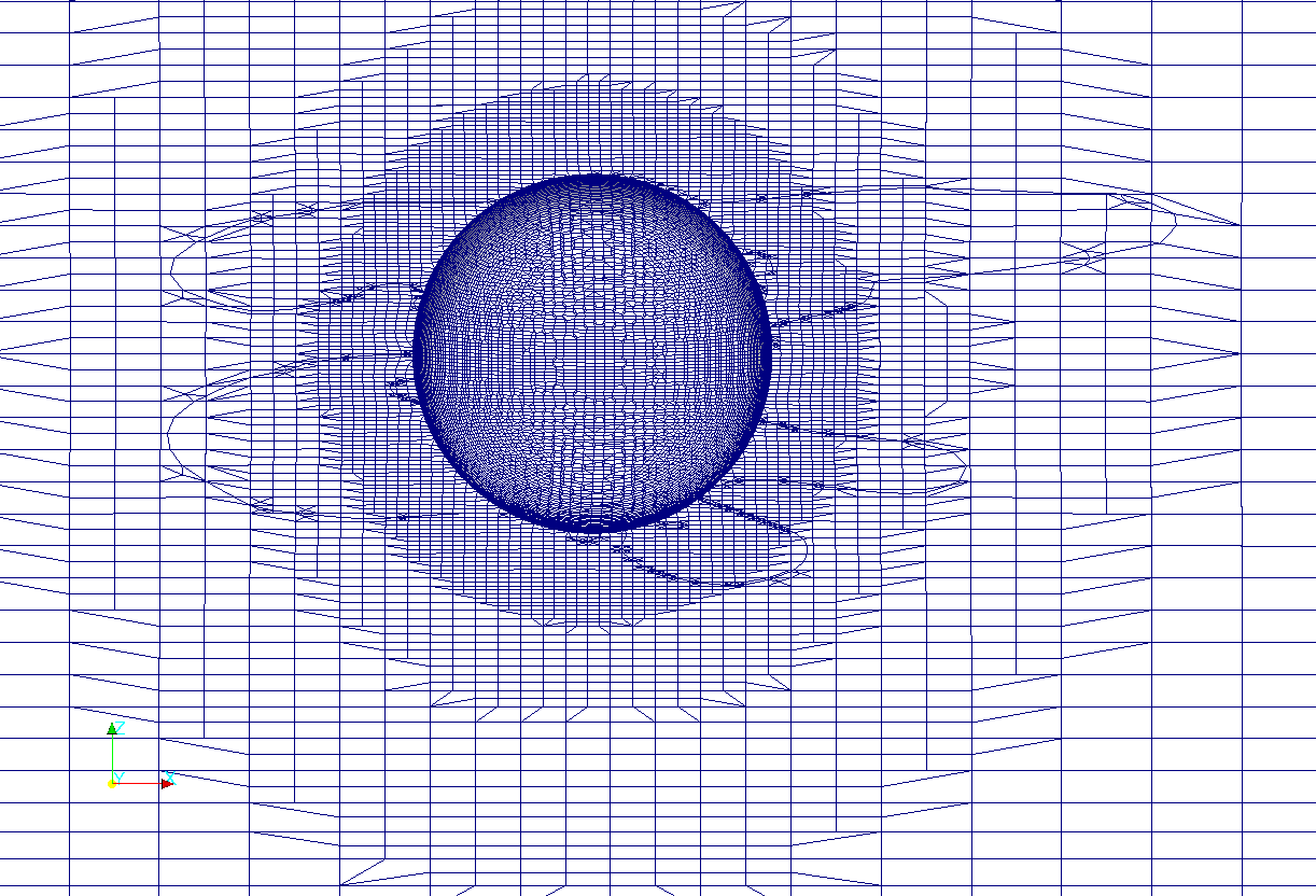
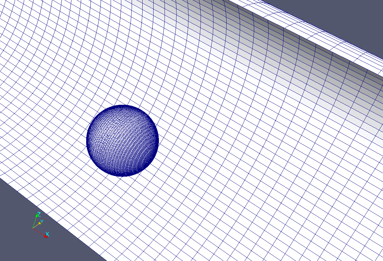
Mesh with internal sphere

Unlike previous time I've decided not to compare turbulence models and just selected realizable k-epsilon.

Flow movies

After running the simulations I've got the following flow movies:

The cylinder in the tube, vorticity



The cylinder in the tube, velocity



The sphere in the tube, vorticity



The sphere in the tube, velocity



As expected after initial flow development I've got quite nice vortices going along the tube.

Probes

Since the movies are not quite enough I've added probes along the axis of the tube to record values of velocity, pressure, and turbulent viscosity during the simulations (this is a fragment of controlDict):

functions
{
    probes
    {
        type            probes;
        functionObjectLibs ("libsampling.so");
        outputControl   timeStep;
        outputInterval  1;
        probeLocations
        (
            (2.47 0 0)
            (2.90 0 0)
            (3.5 0 0)
            (5 0 0)
            (6 0 0)
        );
        fields
        (
            U
            p
            nut
        );
    }
}

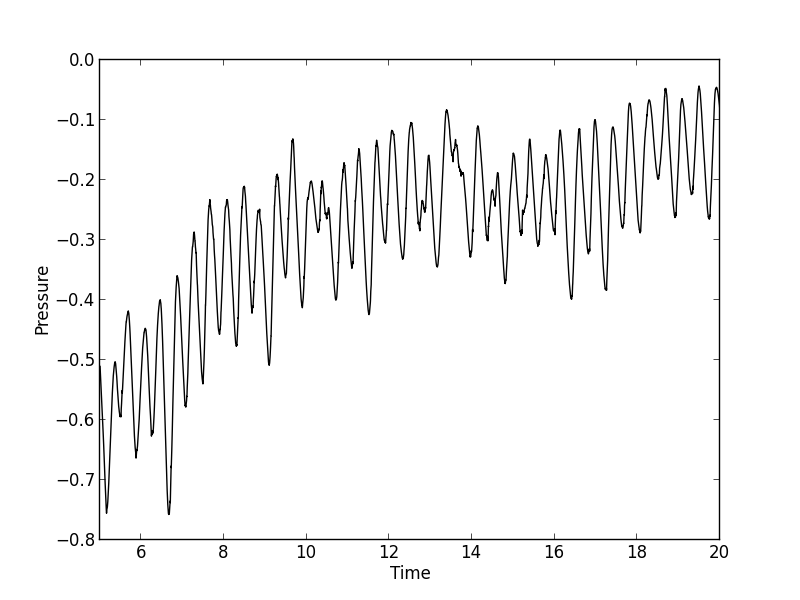
Below is a graphs of the pressure evolution at the location of the first probe (click on the figure for a larger version):

For internal cylinder


For internal sphere


Though evolution has periodic structure but the frequency differs from estimations.

How to run the cases on your own

I've put all necessary files into repository on BitBucket. So you can clone the repo or just download archive of the default branch. There is Cases folder where case files reside. Every case directory has Allprepare script which will do all the necessary utility invocations:

#!/bin/sh
cd ${0%/*} || exit 1

. $WM_PROJECT_DIR/bin/tools/RunFunctions

gmsh - tube.geo
gmsh - cylinder.geo
sed -i -e "s/Created by Gmsh/cylinder/" cylinder.stl
mv cylinder.stl constant/triSurface
gmshToFoam tube.msh
cp -r 0.org 0
changeDictionary
surfaceFeatureExtract
snappyHexMesh -overwrite

The script assumes that you have gmsh in your $PATH and first it creates mesh for tube and cylinder, then corrects STL file created by Gmsh, then places STL files to the directory where sHM will look for it, converts tube mesh to OpenFOAM format, corrects boundary type for walls, and finally runs sHM for final mesh creation. sHM procedure is rather lengthy and needs RAM as the limit on the number of cells is 1500000.